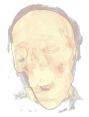
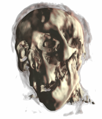
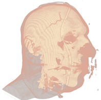
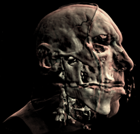
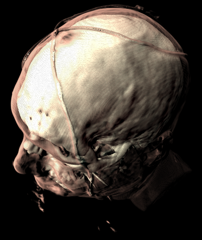
Mummy (top) and Male (bottom) volumes colored with a transfer function (left) and shaded (right).
A transfer function is used to assign RGB and alpha values for every voxel in the volume. A 1D transfer function maps one RGBA value for every isovalue [0, 255]. Multi-dimensional transfer functions allow multiple RGBA values to be mapped to a single isovalue. These are however out of the scope of this tutorial, so I will just focus on 1D transfer functions.
The transfer function is used to "view" a certain part of the volume. As with the second set of pictures above, there is a skin layer/material and there is a skull layer/material. A transfer function could be designed to just look at the skin, the skull, or both (as is pictured). There are a few different ways of creating transfer functions. One is two manually define the transfer functions by specifying the RGBA values for the isovalues (what we will be doing), and another is through visual controls and widgets. Manually defining the transfer function is a lot like guess work and takes a bit of time, but is the easiest way to get your feet wet. Visually designing transfer functions is the easiest way to get good results quickly as it happens at run-time. But this method is quite complex to implement (at least for a tutorial).
Creating the transfer function:
To create a transfer function, we want to define the RGBA values for certain isovalues (control points or control knots) and then interpolate between these values to produce a smooth transition between layers/materials. Our transfer function will result in a 1D texture with a width of 256.
First we have the TransferControlPoint class. This class takes an RGB color or alpha value for a specific isovalue.
public class TransferControlPoint{
    public Vector4 Color;
    public int IsoValue;

    /// <summary>
    /// Constructor for color control points.
    /// Takes rgb color components that specify the color at the supplied isovalue.
    /// </summary>
    /// <param name="x"></param>
    /// <param name="y"></param>
    /// <param name="z"></param>
    /// <param name="isovalue"></param>
    public TransferControlPoint(float r, float g, float b, int isovalue)
    {
        Color.X = r;
        Color.Y = g;
        Color.Z = b;
        Color.W = 1.0f;
        IsoValue = isovalue;
    }

    /// <summary>
    /// Constructor for alpha control points.
    /// Takes an alpha that specifies the aplpha at the supplied isovalue.
    /// </summary>
    /// <param name="alpha"></param>
    /// <param name="isovalue"></param>
    public TransferControlPoint(float alpha, int isovalue)
    {
        Color.X = 0.0f;
        Color.Y = 0.0f;
        Color.Z = 0.0f;
        Color.W = alpha;
        IsoValue = isovalue;
    }
}
This class will represent the control points that we will interpolate. I've added two lists to the Volume class, mAlphaKnots and mColorKnots. These will be the list of transfer control points that we will setup and interpolate to produce the transfer function. To produce the result for the Male dataset above, here are the transfer control points that we will define:
mesh.ColorKnots = new List<TransferControlPoint> {
                        new TransferControlPoint(.91f, .7f, .61f, 0),
                        new TransferControlPoint(.91f, .7f, .61f, 80),
                        new TransferControlPoint(1.0f, 1.0f, .85f, 82),
                        new TransferControlPoint(1.0f, 1.0f, .85f, 256)
                        };

mesh.AlphaKnots = new List<TransferControlPoint> {
                        new TransferControlPoint(0.0f, 0),
                        new TransferControlPoint(0.0f, 40),
                        new TransferControlPoint(0.2f, 60),
                        new TransferControlPoint(0.05f, 63),
                        new TransferControlPoint(0.0f, 80),
                        new TransferControlPoint(0.9f, 82),
                        new TransferControlPoint(1f, 256)
                        };
You need to specify at least two control points at isovalues 0 and 256 for both alpha and color. Also the control points need to be ordered (low to high) by the isovalue. So the first entry in the list should always be the RGB/alpha value for the zero isovalue, and the last entry should always be the RGB/alpha value for the 256 isovalue. The above list of control points produce the following transfer function after interpolation:
So we have defined a range of color for the skin and a longer range of color for the skull/bone.
But how do we interpolate between the control points? We will fit a cubic spline to the control points to produce a nice smooth interpolation between the knots. For a more in-depth discussion on cubic splines refer to my camera animation tutorial.
Here is a simple graph representation of the spline that is fit to the control points.

Using the transfer function:
So how do we put this transfer function to use? First we set it to a 1D texture and upload it to the graphics card. Then in the shader, we simply take the isovalue sampled from the 3d volume texture and use that to index the transfer function texture.
value = tex3Dlod(VolumeS, pos);

src = tex1Dlod(TransferS, value.a);
Now we have the color and opacity of the current sample. Next, we have to shade it. While this is simply diffuse shading I will go over how to calculate gradients (aka normals) for the 3D volume.
Calculating Gradients:
The method we will use to calculate the gradients is the central differences scheme. This takes the last and next samples of the current sample to calculate the gradient/normal. This can be performed at run-time in the shader, but as it requires 6 extra texture fetches from the 3D texture, it is quite slow. So we will calculate the gradients and place them in the RGB components of our volume texture and move the isovalue to the alpha channel. This way we only need one volume texture for the data set instead of two: one for the gradients and one for the isovalues.
Calculating the gradients is pretty simple. We just loop through all the samples and find the difference between the next and previous sample to calculate the gradients:
/// <summary>
/// Generates gradients using a central differences scheme./// </summary>
/// <param name="sampleSize">The size/radius of the sample to take.</param>private void generateGradients(int sampleSize)
{
    int n = sampleSize;
    Vector3 normal = Vector3.Zero;
    Vector3 s1, s2;

    int index = 0;
    for (int z = 0; z < mDepth; z++)
    {
        for (int y = 0; y < mHeight; y++)
        {
            for (int x = 0; x < mWidth; x++)
            {
                s1.X = sampleVolume(x - n, y, z);
                s2.X = sampleVolume(x + n, y, z);
                s1.Y = sampleVolume(x, y - n, z);
                s2.Y = sampleVolume(x, y + n, z);
                s1.Z = sampleVolume(x, y, z - n);
                s2.Z = sampleVolume(x, y, z + n);

                mGradients[index++] = Vector3.Normalize(s2 - s1);
                if (float.IsNaN(mGradients[index - 1].X))
                    mGradients[index - 1] = Vector3.Zero;
            }
        }
    }
}
Next we will filter the gradients to smooth them out and prevent any high irregularities. We achieve this by a simple NxNxN cube filter. A cube filter simply averages the surrounding N^3 - 1 samples. Here's the code for the gradient filtering:
/// <summary>
/// Applies an NxNxN filter to the gradients./// Should be an odd number of samples. 3 used by default./// </summary>
/// <param name="n"></param>private void filterNxNxN(int n)
{
    int index = 0;
    for (int z = 0; z < mDepth; z++)
    {
        for (int y = 0; y < mHeight; y++)
        {
            for (int x = 0; x < mWidth; x++)
            {
                mGradients[index++] = sampleNxNxN(x, y, z, n);
            }
        }
    }
}

/// <summary>
/// Samples the sub-volume graident volume and returns the average./// Should be an odd number of samples./// </summary>
/// <param name="x"></param>
/// <param name="y"></param>
/// <param name="z"></param>
/// <param name="n"></param>
/// <returns></returns>private Vector3 sampleNxNxN(int x, int y, int z, int n)
{
    n = (n - 1) / 2;

    Vector3 average = Vector3.Zero;
    int num = 0;

    for (int k = z - n; k <= z + n; k++)
    {
        for (int j = y - n; j <= y + n; j++)
        {
            for (int i = x - n; i <= x + n; i++)
            {
                if (isInBounds(i, j, k))
                {
                    average += sampleGradients(i, j, k);
                    num++;
                }
            }
        }
    }

    average /= (float)num;
    if (average.X != 0.0f && average.Y != 0.0f && average.Z != 0.0f)
        average.Normalize();

    return average;
}
This is a really simple and slow way of filtering the gradients. A better way is to use a seperable 3D Gaussian kernal to filter the gradients.
Now that we have the gradients we just fill the xyz components of the 3D volume texture and put the isovalue in the alpha channel:
//transform the data to HalfVector4HalfVector4[] gradients = new HalfVector4[mGradients.Length];
for (int i = 0; i < mGradients.Length; i++)
{
    gradients[i] = new HalfVector4(mGradients[i].X, mGradients[i].Y, mGradients[i].Z, mScalars[i].ToVector4().W);
}

mVolume.SetData<HalfVector4>(gradients);
mEffect.Parameters["Volume"].SetValue(mVolume);
And that's pretty much it. Creating a good transfer function can take a little time, but this simple 1D transfer function can still produce pretty good results. Here's a few captures of what this demo can produce:
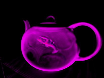
A teapot with just transfer function:

The teapot with transfer function and shaded:


Now a CT scan of a male head. Just transfer function:

Now with shading:




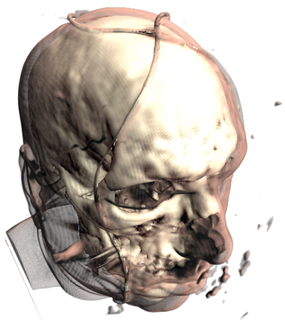
And a mummy:


*The CT Male data set was converted from PVM format to RAW format with the V3 library. The original data set can be found here: http://www9.informatik.uni-erlangen.de/External/vollib/
30 comments:
Thanks for great tutorial!
i've got some problems i don't understand with your source:
Actually Texture3D are not showed)
It have been loaded from file, processed in draw method. But all i can see in the result is wired bounding box...
Do you have any idea why this may appear?
PS: PC config AMD 64 Turion X2(running x86 XP)+ Mobility Radeon x1600(up to 256Mb)
So the RAW file loads just fine? And there aren't any errors?
Did the first demo run for you?
Have you tried just displaying the positions or the Direction (there is a RayCastDirection technique that does this)?
If using the RayCastDirection technique you can display the positions and direction, then it might be an issue with the ATi card not liking the shader.
If you can't display the positions and directions then it is probably a texture format issue.
Hi and thanks for all the great information you have put up.
I am trying to construct a very simple volume renderer, but have recently encountered a problem trying to calculate the gradient for data elements in a dicom image.
I am being throw a Null pointer exception when i try to calculate an individual gradient and write t to an array.
I was wondering if you might have any ideas what the problem could be.
Are you using the sample I provided?
It sounds like you might be overstepping some boundaries. Trying to index outside the array?
Hi, thanks for the help.
I am (foolishly) trying to write my own as part of a project for college.
I was going out of bounds. I was wondering if you had any thoughts about the following.
I am trying to use the central difference equations to calculate a set of gradients for each CT slice.
I read in a dicom file and extract the pixels to a buffered image and then perform the operations. however, i am curious as to how the normalization process would take place on this RGB data. Simply divide by 256(the total number of colors) doesn't seem like it will be that easy.
Thanks
hi, thanks for the great info, i am trying to calculate a set of gradients for a set of images.
I read in the image and save it as a buffered image. i then go about looping through each pixel in the image.
However i am curious if you would know it is possible to do this when dealing with RGB values. i get both pixel in the x-direction say and then....
perform a subtract of the two integer values?? i am unsure
thank you again.
Hi Max,
I'm not quite sure what your problem is. You can still use the central differences scheme using the [0,255] RGB values (However, it may not be as accurate as floating point). Depending on the type of buffer you're writing to, you can keep them in the [0, 255] range or you will need to convert them to [0, 1] floating point range (i.e. for a floating point texture).
To Normalize the data in the [0, 255] range shouldn't be any different than what I have in my code. You simply divide the Gradient vector by its length. Where length is sqrt(R^2 + B^2 + C^2).
Hi Jay,
The data shouldn't need to be in the [0,1] floating point range. You can still use the same algorithms in the project with RGB data.
Unless I'm misunderstanding your question?
Hi,
Could you recommend a good techinque for looking at the texture once it's been exported to png? I've tried a few tools/formats, and have had no luck!
Thanks!
Are you talking about the 3d volume texture?
You can export it as a .dds and use the directx texture tool to look at it. The tool should be included with the directx sdk.
Sorry, I meant the transfer function texture. I saved it as a png using mTransferTex.Save("Content/Textures/transfer.png", ImageFileFormat.Png), and opened it with both gimp and dxtex, but it didn't look like your example. I know it's only one line thick, unlike your representation, and that's no big deal, but the alpha values are not displayed correctly. The first 1/3 or so looks aquamarine, and the second 2/3 is just white...zoomed in 800% that is using dxtex.
Thanks
Ah, ok. That actually sounds about right.
The first third has very low alpha, while the last 2/3 has very high alpha. You can see the difference better using gimp or photoshop than the dx texture tool.
Aquamarine in the dx texture tool means an alpha value of zero or near zero. Which, if you look at the transfer function setup, we're defining very low alpha values for the first third.
Right. My question is, is there a convenient way to view it like you had in the tutorial:
"The above list of control points produce the following transfer function after interpolation: transfer_func[5].png"
In other words, how can I view it as the color you have assigned to it, using the alpha values like your png? Even if only one line!
Thanks
Crap, sorry I meant to mention in my last comment that the image in the tutorial is an artistic representation of what the transfer function should look like.
An easy way to get something similar, is to open it up in gimp and then put a white background behind the texture.
So besides that I don't know an easy way to get a better representation.
Sounds good :) I won't beat myself up trying to figure it out anymore!
Thanks!
Hi,
thanks very much for this excellent series of tutorials, which are a great introduction to the whole area of direct volume rendering.
One thing is puzzling me about this particular tutorial though: I may be wrong, but it seems like you're using a 1D Cubic interpolation method on to generate the alpha for your transfer function, where mu is mapped directly to the x axis of the the 1D texture. I'm hazy on the maths involved, but from my own experiments, and from reading
http://local.wasp.uwa.edu.au/~pbourke/miscellaneous/interpolation/ it seems that 1D cubic interpolation would only produce a smooth curve if the points are equally-spaced along the x-axis. I'm on a Mac, so unfortunately I can't easily compile your your example project to see how it works in practice I'd be intrigued to know if you'd considered this issue. It could be that in this context it's not a problem.
Thanks again,
Alex
Perhaps if it was simply a cubic interpolation, it would not produce a smooth curve. However, the sample fits a natural cubic spline to the alpha/color knots and so should produce a smooth curve. Though I'm no expert.
In any case, it isn't really a big deal if the curve isn't totally smooth, as in most cases you wouldn't notice it in the transfer function. In fact most use simple linear interpolation to produce transfer functions. Actually a cubic spline in this case is a bit overkill :P
You're right- I'm sure in practice it doesn't matter, but I'm pretty certain that a 1D cubic spline doesn't porduce a smooth curve unless the data point are equally-spaced along the x-axis.
Here's a couple of examples:
http://mcserver.gold.ac.uk/temp/cubicspline-2-3.png
http://mcserver.gold.ac.uk/temp/cubicspline-2-4.png
You can see some fairly sharp corners where points are close together.
I know it doesn't really matter in this context, but it's really bugging me now. There must be a way of creating a smooth curve where the points are not equally-spaced....
Anyway, thanks again for the excellent tutorial.
a|x
nice article, thanks.
machinesdontcare: sure there is. ever seen curves in photoshop? they use so-called cubic spline interpolation. take a look at this for instance
http://www.codeproject.com/KB/cs/SplineInterpolation.aspx?msg=1508968
or this
http://mathworld.wolfram.com/LagrangeInterpolatingPolynomial.html
the second one is more ugly (too wavy if you use too many control points), but extremely easy to understand and implement. the first link contains this as well if i'm not wrong, i just googled it and haven't examined it too much.
Thanks for these volume rendering posts. I found them very useful.
Hi kyle
I have already rendered my volume, I want to create a function for to generate the transfer function. You talk about 256 - 1D texture, then talk about the control points, my question is: How I generate the 256 rgba samples colors and how to combine the control points into the texture 1D?. I need one texture or 2 textures ?
Thanks,
Jos
To generate the transfer function you setup the control points and interpolate between them. These act as the points of interest inside the volume. So for every pixel of the transfer function texture, you sample the control point curve to find the value for the pixel.
Thanks for your help. Has any standard to assign a determine color (transfer function) a to human body ?
Jos
Hey,
Thanks for the excellent articles, they really helped when I was programming my own volume renderer!
As you were kind enough to share your experiences, I tried to return the favor and I've posted a sort of follow-on article on some other optimizations you can do for volume rendering.URL below
http://www.marcusbannerman.co.uk/index.php/home/42-articles/97-vol-render-optimizations.html
Thanks,
Marcus
Hi Kyle,
very nice tutorial! I've ported it to DirectX 11 just for fun (source code and binary files available at http://christian.mendl.net/pages/software.html)
Hi,
Thanks for the awesome tutorial, I have one question so what exactly is the rule of the opacity function?
Hi Lily,
I'm not quite sure what you mean by rule. Do you mean what is a general guideline in designing the opacity/transfer function?
As the post outlines, the transfer function maps a single scalar value to a color and opacity. As far as picking colors and alpha values for specific isovalues of the data set, that just requires some experimentation.
In the case of the head model, we want the skin to be transparent over the opaque bone underneath, so we choose values that accomplish this.
As far as color, you generally want to stay in the displayable range of colors (unless you're tonmeapping), so our transfer function is clamped to [0,255] rgb values.
Hope that helps,
Kyle
Hi Kyle,
That helps a lot, Thanks!! Your tutorial answered a question that I have been having for a long time.
Great blog!!
Thanks for the great explanation!!
Can you please load the RAW data, or explain how to upload the data to your code please?
I need some medical data to use in my class.
Thanks!
-LM
Hi LM,
I'm not entirely sure of your question. The data used in the demo is already in the RAW format.
You can find the original dataset here: http://www9.informatik.uni-erlangen.de/External/vollib/
Which also contains a link to the V^3 library that you can use to convert the datasets to RAW format.
Post a Comment